Cost of Production and Break Even Price Analysis (2020/21)

The average budgeted unit Cost of Production (before interest), and Break Even Price (after interest), calculated from 2020/21 client budgets for the major commodities is shown below:

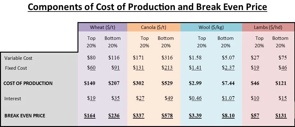
The Cost of Production (COP) and Break Even Prices (BEP) have fluctuated dramatically from the figures calculated for 2019/20. Both the COP and BEP prices are significantly greater for clients in the bottom 20% than those in the top 20%. This highlights the producers who effectively allocate inputs to achieve their economic yield potential.

Caution is required in interpreting these figures, as no two businesses are the same and the sample size is relatively small for comparison purposes. However, the figures do show what is achieved by some clients, plus the extent of their comparative advantage in a competitive marketplace, both locally and globally.

Due to the tough seasonal conditions experienced in the last two seasons, many clients have altered their production system to reduce risk from dry conditions. This includes a significant increase in the proportion of cereal crops, particularly barley at the expense of canola in western areas. Clients who run livestock have also increased their stock numbers, to capitalise on robust returns. Other clients have cut costs dramatically, particularly fertiliser, due to reduced nutrient removal over the last few years.

Rising soil Phosphorous levels to luxurious numbers reflects the use of higher than removal application rates, while higher rates of chemicals are being used to combat herbicide resistance.

Costs attributed to wool have declined due to the decrease in the price of wool relative to lambs, which results in a reallocation of costs.

The top 20% of producers continue to have both lower variable and fixed unit costs than the bottom 20%, due to higher productivity and better matching of variable costs to expected output.

The challenge to management is to achieve a Cost of Production which provides sufficient margin from expected commodity returns.  The suggested target margin is at least 25% of expected returns.

Therefore if the net ESR for wheat is $250/tonne, the desired Cost of Production is $188/tonne or less.  For lambs, if $120/head net is obtained, the Cost of Production needs to be $90/head or less to achieve a 25% margin on sales.

The unit cost of production for the top 20% of wheat and canola producers, is around 67% and 57% respectively of that for the bottom 20% of producers, while the unit cost of production for the top 20% of wool and lamb producers, is about 40% and 38% respectively of that for the bottom 20% of these producers.

The top 20% of client producers based on Break Even Price, tend to have lower interest costs per unit of output, along with lower variable and fixed costs, compared with the bottom 20% of producers.

An example of the differences in unitised variable, fixed and interest costs between the top 20% and bottom 20% of producers (ranked by total costs), is illustrated in the following table:

The budgeted costs for the top 20% and bottom 20% of clients ranked by total costs per hectare are as follows:

The average total costs of $382/ha for the top 20% of clients ranked on total costs per hectare, is 77% of the overall average of $499/ha. The average interest cost of $49/ha for the top 20% of clients ranked on total costs per hectare, is 84% of the overall average of $58/ha. The average interest cost per hectare for the top 20% has risen by 32% over the last 12 months, while the average interest cost per hectare has fallen by 8%.

This may be due to the 2018 and 2019 droughts impacting on working capital reserves, requiring large businesses to obtain additional finance, or alternatively they are funding land acquisitions.

At the same time significantly reduced interest rates have reduced interest costs for those not borrowing additional funds.

The top 20% group run very large, lean operations in low rainfall environments, with generally low inputs due to lower targeted output, but in line with environmental expectations. During average seasonal conditions they often reduce debt quickly from higher operating surpluses, then re-borrow to expand again through land purchases.